Alisa Knizel
Alisa Knizel
Yizhen Li
Yizhen Li

Breaking Universality
in Dimer Models

Leonid Petrov

University of Virginia

Joint work with Alisa Knizel (Barnard / Columbia) arXiv:2507.22011 (opens in new tab)
and Alexey Bufetov, Panagiotis Zografos (Leipzig) arXiv:2507.08560 (opens in new tab)

Alexey Bufetov
Alexey Bufetov
Panagiotis Zografos
Panagiotis Zografos
NSF Simons Foundation
lpetrov.cc/lozenge-draw/
Draw a shape and tile by lozenges
QR code for lpetrov.cc/lozenge-draw/
Loading...

Part I

Brief Survey of Universality in Dimer Models

Random Discrete Surfaces

surface in 4 × 12 × 9 box
Theorem [MacMahon, c. 1900]:
Number of surfaces in \(a \times b \times c\) box is \(\displaystyle\prod_{i=1}^{a}\prod_{j=1}^{b}\prod_{k=1}^{c}\frac{i+j+k-1}{i+j+k-2}\)
For 9 × 12 × 9: 1,340,992,301,315,806,672,824,460,528,012,500
... and we pick one at random from this collection
How does a typical random surface look like, depending on the boundary?

Other Ways to Build 3D Surfaces

4 non-flat building blocks instead of 3 flat squares.
General theory for planar bipartite dimer models: [Kenyon–Okounkov–Sheffield 2006]
Glue into a surface.
The top-down view is a domino tiling of the Aztec diamond.
We will discuss domino tilings with random edge weights

Limit Shape in 3D

pre-sampled
Theorem [Cohn–Kenyon–Propp 2000]:
As the mesh size → 0, the random stepped surface concentrates around a deterministic limit shape. It develops flat and curved parts.
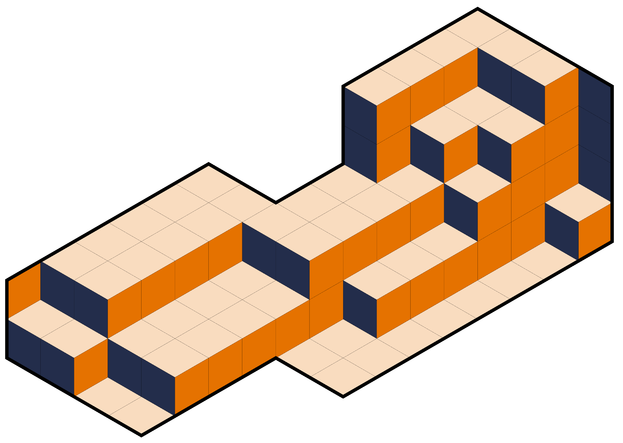
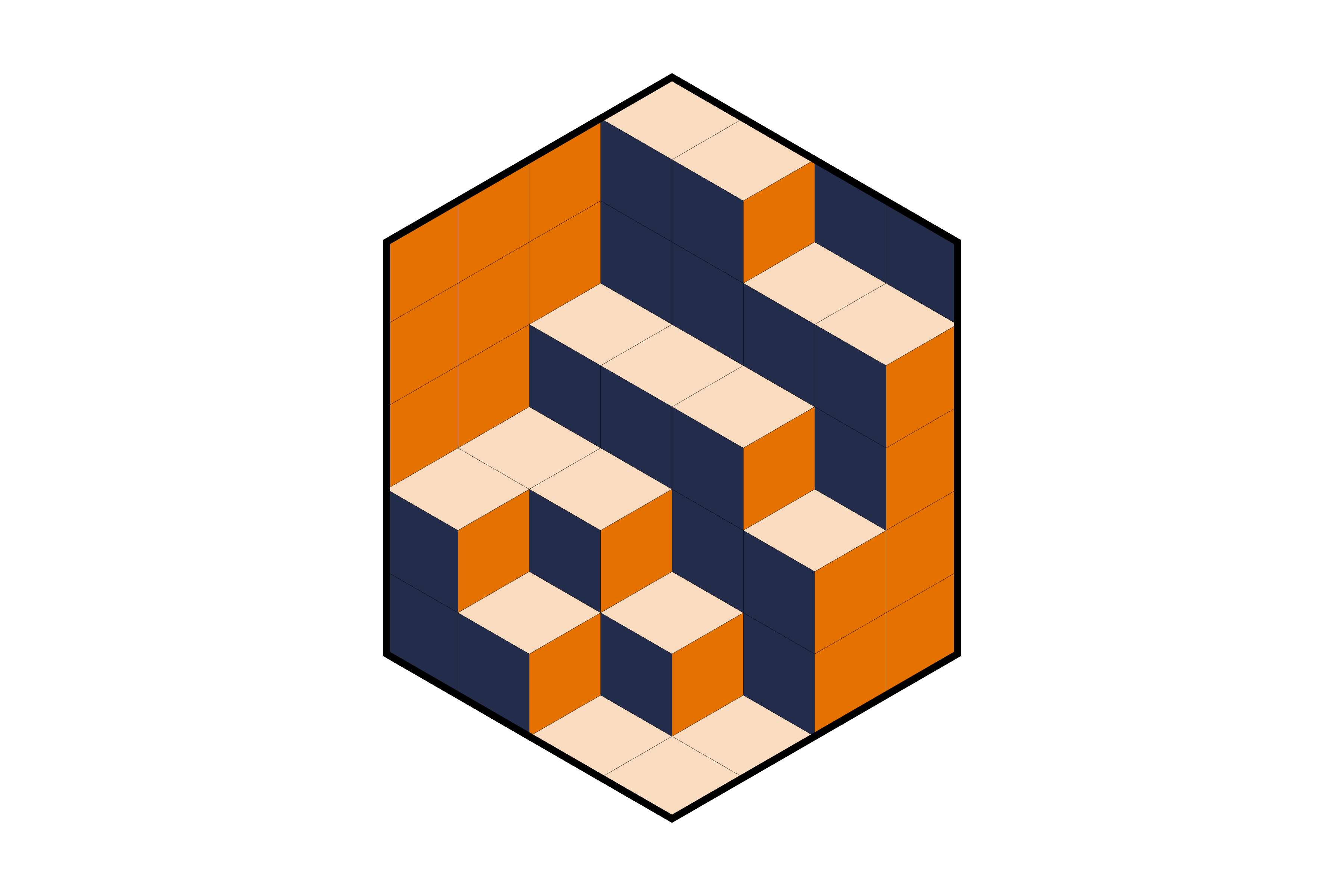
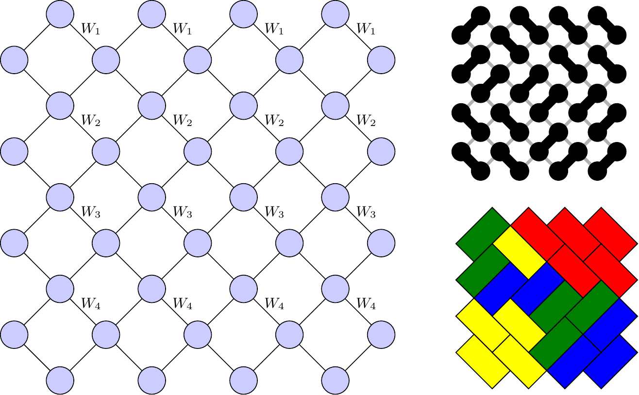
3D surfaces projected to \(x+y+z=0\) are lozenge tilings with three types of lozenges.
Small lozenge tiling as stepped surface

Local Patches

Local patches:
  • Approximate the surface by piecewise-planar patches
  • Each patch is a flat random surface with a given slope \((s_1, s_2)\)
  • For a given slope, the number of approximating 3D surfaces is \(\approx e^{N^2\cdot \sigma(s_1,s_2) }\)
Variational principle [Cohn–Kenyon–Propp 2000]:
Limit shape \(z=h(x,y)\) maximizes \[\displaystyle\iint \sigma(\nabla h)\, dxdy\] subject to boundary conditions on \(h(x,y)\)
\(\sigma(s_1,s_2) = \tfrac{1}{\pi}\bigl[\Lambda(\pi s_1) + \Lambda(\pi s_2) + \Lambda(\pi (1\!-\!s_1\!-\!s_2))\bigr]\)
\(\Lambda(\theta)=-\!\int_0^\theta \ln|2\sin t|\,dt\)   (Lobachevsky function)
Other 3D building blocks besides squares of three directions: [Kenyon–Okounkov–Sheffield 2006]
plane z=Ax+By

Universality: Zoom In

Zoom in around any point in the liquid region → same class of universal local statistics determined only by slope (ergodic translationally invariant Gibbs measures on tilings of the full plane - pure states)
Determinantal point process in 2D:
\[\rho_k\bigl((t_1,x_1),\ldots,(t_k,x_k)\bigr) = \det\bigl[K(t_i,x_i; t_j,x_j)\bigr]_{i,j=1}^{k}\]
= probability to find non-blue lozenges at each \((t_i, x_i)\)
Incomplete Beta kernel:
\[K_u(t,x;s,y) = -\frac{1}{2\pi\mathbf{i}} \int_{\bar{u}}^{u} (1-z)^{t-s} z^{-(x-y)-1} dz\]
[Okounkov–Reshetikhin '01], [Sheffield '03], [Kenyon–Okounkov–Sheffield '03], [Gorin '07], [P. '12], [Gorin–P. '16], [Aggarwal '19]
pre-sampled
Local structure at different slopes in the liquid region

Height Fluctuations

Gaussian Free Field
Like the Brownian bridge, but with two-dimensional time
\(\displaystyle \text{GFF} \approx \frac{h_1 - h_2}{\sqrt{2}}\)
where \(h_1, h_2\) are two independent samples of the height function.
Covariance structure:
The complex coordinate \(u\colon\) liquid region \(\to\) upper half plane \(\mathbb{H}\) determines the correlations:
\(\displaystyle \operatorname{Cov}(h(x_1), h(x_2)) \to -\frac{1}{2\pi^2} \ln\left|\frac{u(x_1)-u(x_2)}{u(x_1)-\bar u(x_2)}\right|\)
= Green function on \(\mathbb{H}\), pulled back by \(u\)
Fluctuations of the height function are \(O(\sqrt{\log N})\). Correlations stay bounded as \(N \to \infty\). Universality is open even for simply connected domains.
[Kenyon 2001], [Kenyon 2008], [Petrov 2014], [Berestycki–Laslier–Ray 2020], [Bufetov–Gorin 2018], [Borot–Gorin–Guionnet 2026]

Universality: Domino Tilings

Same GFF for domino tilings
Height fluctuations of random domino tilings of the Aztec diamond converge to the Gaussian Free Field — same universality class as lozenge tilings
Covariance: pulled back by conformal map \(u\) to \(\mathbb{H}\), same Green function structure
[Kenyon 2001], [Bufetov–Knizel 2018], [Chelkak–Laslier–Russkikh 2020], [Berggren–Nicoletti–Russkikh 2024]

Summary So Far

Limit shapes. Random 3D surfaces have deterministic limit shapes as the mesh size \(\to 0\).
Local universality. At the lattice level, local statistics display universal behavior (translation-invariant Gibbs measures determined by slope).
Global universality. Globally, height fluctuations are described by the Gaussian Free Field.
Edge behavior / KPZ. At the boundary between frozen and liquid regions, fluctuations are governed by the Airy line ensemble — the same universal object appearing throughout the \((1+1)\)-dimensional KPZ universality class (TASEP, last-passage percolation, directed polymers, \(\ldots\)).
Not covered in this talk — but central to many other talks at this conference.

Part II

The Waterfall

Breaking Local Universality in Lozenge Tilings

with Alisa Knizel arXiv:2507.22011 (opens in new tab)

Q-volume deformation

q =
q =
q =
q =
q =
\(\displaystyle \text{Prob}(\text{surface}) = \frac{q^{\text{volume under surface}}}{\sum_{\text{all surfaces}} q^{\text{volume}}}\)
Variational principle (\(q = e^{-\gamma/N}\))
Maximize \(\displaystyle \iint \sigma(\nabla h) \, dx\,dy - \gamma \iint h \, dx\,dy\)
\(\gamma>0\): less volume  ·  \(\gamma<0\): more volume
On the hexagon: related to q-Hahn orthogonal polynomials. Not the most general basic hypergeometric family...
For \(q = e^{-\gamma/N} \to 1\): expect the same universal local behavior (pure states with incomplete Beta kernel locally, and GFF fluctuations globally) — but less is proven

More deformation: q-Racah tilings of the hexagon

Orthogonal polynomials:
Classical: Hermite, Laguerre, Jacobi, Legendre, ...
if you ask for explicit coefficients, you can climb up to q-discrete ("exotic") world. The ladder is the (q-)Askey scheme
At the very top: q-Racah polynomials
Exactly solvable measure on boxed surfaces (hexagon tilings) discovered by [Borodin-Gorin-Rains 2009], connected to the q-Racah polynomials
\[ \mathbb{P}(\text{tiling}) = \frac{1}{Z} \prod_{\substack{\text{horiz.}\\\text{lozenges}}} \mathrm{w}(h),\qquad \mathrm{w}(h) = \chi\, q^{h} + \frac{1}{\chi\, q^{h}} \]
\(h\) — height, centered around the middle of the hexagon
\(q \in (0,1]\) — volume tilt,   \(\chi > 0\) — interpolation parameter
\(\chi \to 0\) gives \(q^{-\text{vol}}\),   \(\chi \to +\infty\) gives \(q^{+\text{vol}}\)
Results [BGR 2009], [Dimitrov-Knizel 2019], [Gorin-Huang 2022], [Duits-Duse-Liu 2023]:
Same local limits (pure states) and GFF fluctuations as \(q = e^{-\gamma/N}\), but different limit shape
Lozenge tiling of a hexagon
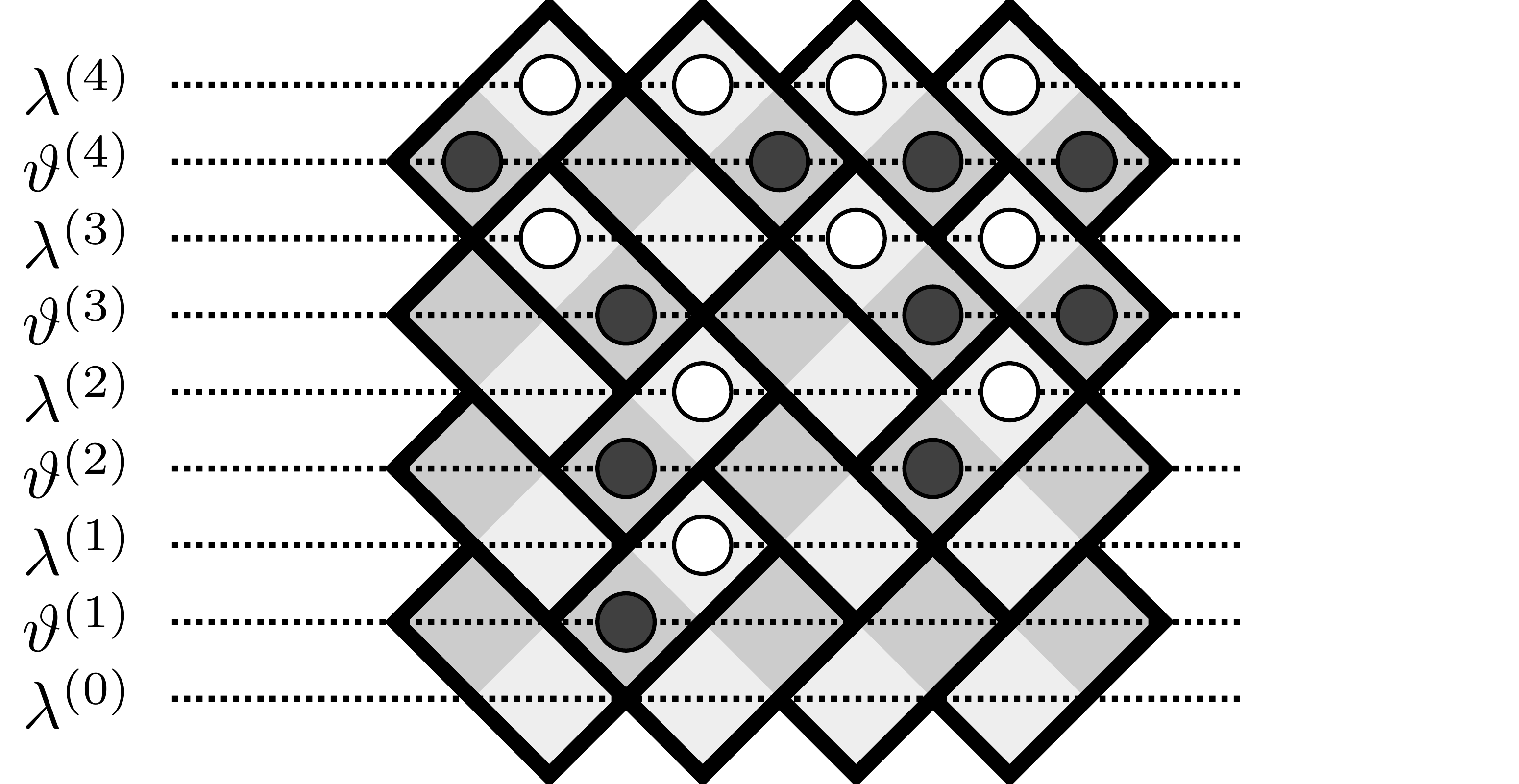
Example. Counting horizontal lozenges by centered height:
\(h = -2.5\):3
\(h = -1.5\):2
\(h = -0.5\):4
\(h = \phantom{-}0.5\):3
\(h = \phantom{-}1.5\):2
\(h = \phantom{-}2.5\):2
Particles in two dimensions in a double-well potential

q-Racah Tilings of Large Hexagons

\(q = 0.95\), \(\chi = 3\)
\(q = 0.8\), \(\chi = 3\)
When \(q = e^{-\gamma/N} \to 1\): curved limit shape and the same universal local fluctuations (pure states with the incomplete Beta kernel) as for the uniform and q-volume measures [Borodin-Gorin-Rains 2009].

Global fluctuations:
[Dimitrov-Knizel 2019], [Gorin-Huang 2022], [Duits-Duse-Liu 2023]
But since 2009, it was not clear what happens for fixed \(q\). This became known as the waterfall phenomenon.

The Waterfall: Dimensional Collapse [Knizel-P. 2025]

Theorem [Knizel-P. 2025, arXiv:2507.22011]
Probability to find a horizontal (light-colored) lozenge in the waterfall region is exponentially small:
\(\mathbb{P}(\text{horizontal lozenge}) \sim e^{-cN}\)
Why? \(\displaystyle\mathrm{w}(h) = \chi\, q^{h} + \frac{1}{\chi\, q^{h}}\) \(\to\) avoid center
Classical regime \(q = e^{-\gamma/N} \to 1\):
  • frozen/semifrozen (no randomness but regular pattern of one or two colors)
  • or liquid/gaseous (all three colors present; phases differ by correlation decay)

q-Racah Orthogonal Polynomial Ensemble

Lozenge tiling and paths

Vertical slice \(\to\) \(N\) noncolliding paths

Correlation kernel:
\(\displaystyle K_t(x, y) = \sum_{n=0}^{N-1} f_n^t(x) f_n^t(y)\)
\(f_n^t\): orthonormal q-Racah polynomials on slice \(t\)
\(K_t\): spectral projection for q-difference operator
Key observation [Borodin-Gorin-Rains 2009]
The marginal distribution of paths on a vertical slice is the q-Racah orthogonal polynomial ensemble. This is basically how the deformation was discovered.
Joint distribution:
\(\displaystyle \mathfrak{R}^{qR(N)}_{M,\alpha,\beta,\gamma,\delta}(x_1, \ldots, x_N) = \frac{1}{Z} \prod_{1 \le i < j \le N} (\mu(x_i) - \mu(x_j))^2 \prod_{i=1}^N w^{qR}(x_i)\)
where \(\mu(x) = q^{-x} + \gamma\delta q^{x+1}\)
Weight function:
\(\displaystyle w^{qR}(x) := \frac{(\alpha q; q)_x (\beta\delta q; q)_x (\gamma q; q)_x (\gamma\delta q; q)_x}{(q; q)_x (\alpha^{-1}\gamma\delta q; q)_x (\beta^{-1}\gamma q; q)_x (\delta q; q)_x} \cdot \frac{(1 - \gamma\delta q^{2x+1})}{(\alpha\beta q)^x (1 - \gamma\delta q)}\)
\(\displaystyle (a; q)_k := (1-a)(1-aq) \cdots (1-aq^{k-1})\) is the q-Pochhammer symbol
Parameters: \((M; \alpha, \beta, \gamma, \delta; q, \chi)\), \(\gamma = q^{-M-1}\)
\(\displaystyle M = t + N - 1,\ \alpha = q^{-S-N},\ \beta = q^{S-T-N},\ \gamma = q^{-t-N},\ \delta = -\chi^2 q^{-S+N}\)
Correlations: \(\displaystyle \mathbb{P}(\text{particles at } p_1, \ldots, p_m) = \det\bigl[K_t(p_i, p_j)\bigr]_{i,j=1}^{m}\)

Local Limit for Fixed q

q-Difference operator: \(B(x), D(x)\) are explicit rational expressions in factors like \((q^T + \chi^2 q^{x+1})\),
\(\displaystyle (\mathfrak{D}^{qR}g)(x) := \sqrt{\frac{w^{qR}(x)}{w^{qR}(x+1)}}B(x)\,g(x+1) - [B(x)+D(x)]\,g(x) + \sqrt{\frac{w^{qR}(x)}{w^{qR}(x-1)}}D(x)\,g(x-1)\)
Correlation kernel:
\(\displaystyle K_t(x, y) = \sum_{n=0}^{N-1} f_n^t(x) f_n^t(y)\)
\(f_n^t\): orthonormal q-Racah polynomials on slice \(t\)
Kernel = projection onto spectral interval:
\(\displaystyle \bigl[-q^{-N+1}(1-q^{N-1})(q^{-T-N}-1),\, 0\bigr]\)
  • [Reed-Simon 1972] Then spectral projections (kernels) converge!
  • [Olshanski 2008] spectral projections for determinantal processes, [Tao 2011] nonrigorous application to random matrices
  • [BGR 2009] extension to 2D correlations - not much difference with 1D when \(q=e^{-\gamma/N}\to 1\)
As \(T,S,N,x,t \to \infty\) proportionally while \(q = e^{-\gamma/N} \to 1\):
Coefficients behave nicely. Difference operators converge to
\(\displaystyle f \mapsto \tfrac{1}{2}(f(x+1) + f(x-1)) - c\,f(x)\)
Limiting spectral projection (onto \(\geq 0\)) is multiplication by \(\mathbf{1}_{\mathrm{Re}(z) > c}\)
Inverse Fourier \(\Rightarrow\) discrete sine kernel:
\(\displaystyle K^{\mathrm{sine}}_\phi(x; y) = \frac{\sin(\phi(x-y))}{\pi(x-y)}\)
frozen

Spectral Approach on Vertical Slices?

Question:
What do we expect of the kernel on a vertical slice? Sine kernel limit?
Answer: No.
We expect it to converge to the identity or the zero operator thanks to our result on path concentration [Knizel-P. 2025]
Can we achieve this by taking the spectral approach?
\(\displaystyle (\mathfrak{D}^{qR}g)(x) := \sqrt{\frac{w(x)}{w(x+1)}} B(x) g(x+1) - [B(x)+D(x)] g(x) + \sqrt{\frac{w(x)}{w(x-1)}} D(x) g(x-1)\)
We compute limiting operators. "Nice" only outside the waterfall and at the central point
Example: \(\displaystyle (Tf)(x) = \chi^2\bigl( q^{2x+\frac{3}{2}}f(x+1) + (1+q)q^{2x+1}f(x) + q^{2x+\frac{1}{2}}f(x-1) \bigr),\qquad x\in \mathbb{Z}\)
Problem:
  • Limiting operator is symmetric but not self-adjoint (deficiency indices \((1,1)\))
  • Self-adjoint extension is not unique — spectrum may depend on position in the slice
  • Path concentration already gives the answer inside the waterfall region — no need for spectral analysis unless we want to study the waterfall edge

Spectral Approach in the Transversal Direction

The 2d (extended) correlation kernel is [Borodin–Gorin–Rains 2009]
\(\tilde{K}(s,x;t,y) =\)
\((U_t^{-1}U_{t+1}^{-1}\ldots U_{s-1}^{-1})_y K_s(x,y),\) \(s > t;\)
\(K_t(x,y),\) \(s = t;\)
\((U_{t-1}\ldots U_{s+1}U_s)_y (-\mathbf{1}_{x=y} + K_s(x,y)),\) \(s < t.\)
Relies on inter-slice operators (whose coefficients are explicit and product-form)
\(\displaystyle \tilde{C}_n^t f_n^{t+1}(x) = \sqrt{\frac{\tilde{w}_t(x-1)}{\tilde{w}_{t+1}(x)}} f_n^t(x-1) a_1^t(x-1) + \sqrt{\frac{\tilde{w}_t(x)}{\tilde{w}_{t+1}(x)}} f_n^t(x) a_0^t(x) =: (U_t f_n^t)(x)\)
Inter-slice operators \(U_t\) converge (under our scaling of the hexagon, and for fixed \(q\)), to the following explicit operator on \(\frac12\mathbb{Z}\):
\(\displaystyle \mathfrak{a}(x) \mathcal{F}_n\left(x - \tfrac{1}{2}\right) + \mathfrak{a}\left(x + \tfrac{1}{2}\right) \mathcal{F}_n\left(x + \tfrac{1}{2}\right) = -q^n \mathcal{F}_n(x), \qquad \qquad \mathfrak{a}(x) := \left[\frac{\chi^2 q^{2x-1}}{(1+\chi^2 q^{2x})(1+\chi^2 q^{2x-1})}\right]^{1/2}.\)
Limit operator:
A "very bounded" operator on \(\ell^2(\frac12\mathbb{Z})\): coefficients \(\mathfrak{a}(x)\) rapidly decay as \(|x| \to \infty\).
Key obstacle:
Its inverse (required for the kernel) is "very unbounded"

Inter-slice Operators and Their Limits

  • Put the physics hat on.
  • Diagonalize the limiting \(U_t\) into orthonormal eigenfunctions
  • Pretend that the inverse operator makes sense, and write down the barcode density \(\rho(t)\)
We get a guess:
\(\displaystyle \rho(t) = \mathfrak{a}\bigl(1-\tfrac{t}{2}\bigr) \sum_{n \in \frac{1}{2}\mathbb{Z}_{\geq 0}} \frac{-q^{-n} \mathcal{F}_n^t(0) \mathcal{F}_n^{t-1}(0)}{\|\mathcal{F}_n\|_{\ell^2(\mathbb{Z})}^2}\)
  • How good is the guess?
  • But... this series does not even converge
  • Series diverges "mildly", as \(+c-c+c-c+c-\ldots\)
...And, the barcode process is indeed two-periodic! Taking only even and only odd partial sums, we get two different limits \(\rho_0, \rho_1\) (independent of \(t\)), with \[\rho_0 + \rho_1 = 1\] (corresponds to the waterfall's slope in the \(xy\)-plane). The sums \(\rho_0\) and \(\rho_1\) match the two barcode densities.
\(\displaystyle \mathcal{F}_n(x) := \sqrt{1 + \chi^{-2} q^{-2x}} \sum_{i=-n}^{n} \frac{(-1)^{n+i} q^{-i/2}}{(q;q)_{n-i}(q;q)_{n+i}} \cdot \frac{1}{\theta_{\sqrt{q}}\bigl(\chi q^{x+i+\frac{1}{2}}\bigr)}\)
\(\displaystyle \mathcal{F}_n^t(x) := \mathcal{F}_n\bigl(x - \tfrac{t-1}{2}\bigr)\)
\(\displaystyle (U_t \mathcal{F}_n^t)(x) = -q^n \mathcal{F}_n^{t+1}(x),\qquad \qquad t, x \in \mathbb{Z}, \quad n \in \tfrac{1}{2}\mathbb{Z}_{\geq 0}\)
\(\displaystyle \mathfrak{a}(x) := \left[\frac{\chi^2 q^{2x-1}}{(1+\chi^2 q^{2x})(1+\chi^2 q^{2x-1})}\right]^{1/2}\)
\(\displaystyle \theta_{\sqrt{q}}(z) := (z;\sqrt{q})_\infty (\sqrt{q}/z;\sqrt{q})_\infty\)
(pre-limit)
\(t\) \(\hat{K}^{\mathrm{barcode}}_{(L)}(t,t)\)
−50.5598645425
−40.4388625943
−30.5609384574
−20.4388797292
−10.5610918461
00.4388821809
10.5611137582
20.4388825313
30.5611168883
40.4388825813
50.5611173341
(sum up to \(M\))
\(t\) \(\mathcal{K}^{\mathrm{barcode}}_{(M)}(t,t)\)
−50.5611174103
−40.4388825896
−30.5611174103
−20.4388825896
−10.5611174103
00.4388825896
10.5611174103
20.4388825896
30.5611174103
40.4388825896
50.5611174103

Why 2-Periodic?

Barcode Kernel Conjecture [Knizel-P. 2025]

Conjecture [Knizel-P. 2025]
There exists a barcode kernel \(\mathcal{K}^{\mathrm{barcode}}(s,t)\) governing the limiting determinantal point process. For \(s \ge t\):
\(\displaystyle \mathcal{K}^{\mathrm{barcode}}(s,t) = \lim_{M\to\infty} q^{(M+1)(s-t)} (-1)^{t-s} \sqrt{\frac{\chi^2 q^{1-s}}{(1+\chi^2 q^{2-t})(1+\chi^2 q^{1-s})}} \sum_{n=0}^{M+\frac{1}{2}} \frac{(-q^n)^{t-1-s} \mathcal{F}_n^s(0) \mathcal{F}_n^{t-1}(0)}{\|\mathcal{F}_n\|^2}.\)
For \(s < t\), extend by symmetry: \(\mathcal{K}^{\mathrm{barcode}}(s,t) = \mathcal{K}^{\mathrm{barcode}}(t,s).\)
Properties:
  • The full kernel is two-periodic (2×2 block structure)
  • Agrees with simulations
  • Agrees with numerical limits from pre-limit formulas
Proved [Knizel-P. 2025]:
  • Waterfall exists: path concentration, dimensional collapse to 1D
  • Open since [BGR 2009]
Conjectural:
  • The explicit barcode kernel formula (supported by numerics and simulations)
  • Work in progress with my PhD student Yizhen Li: approach to waterfall and edge-waterfall correlations via another model

Part III

Random Edge Weights

Breaking Global Universality in Domino Tilings

with Alexey Bufetov and Panagiotis Zografos arXiv:2507.08560 (opens in new tab)

Related:
Q. Moulard, F. Toninelli arXiv:2507.11964, Dimers with layered disorder
P. Zografos arXiv:2510.11846, Quenched and Annealed CLTs for the one-periodic Aztec diamond in random environment
M. Duits, R. Van Peski arXiv:2512.03033, The Gamma-disordered Aztec diamond

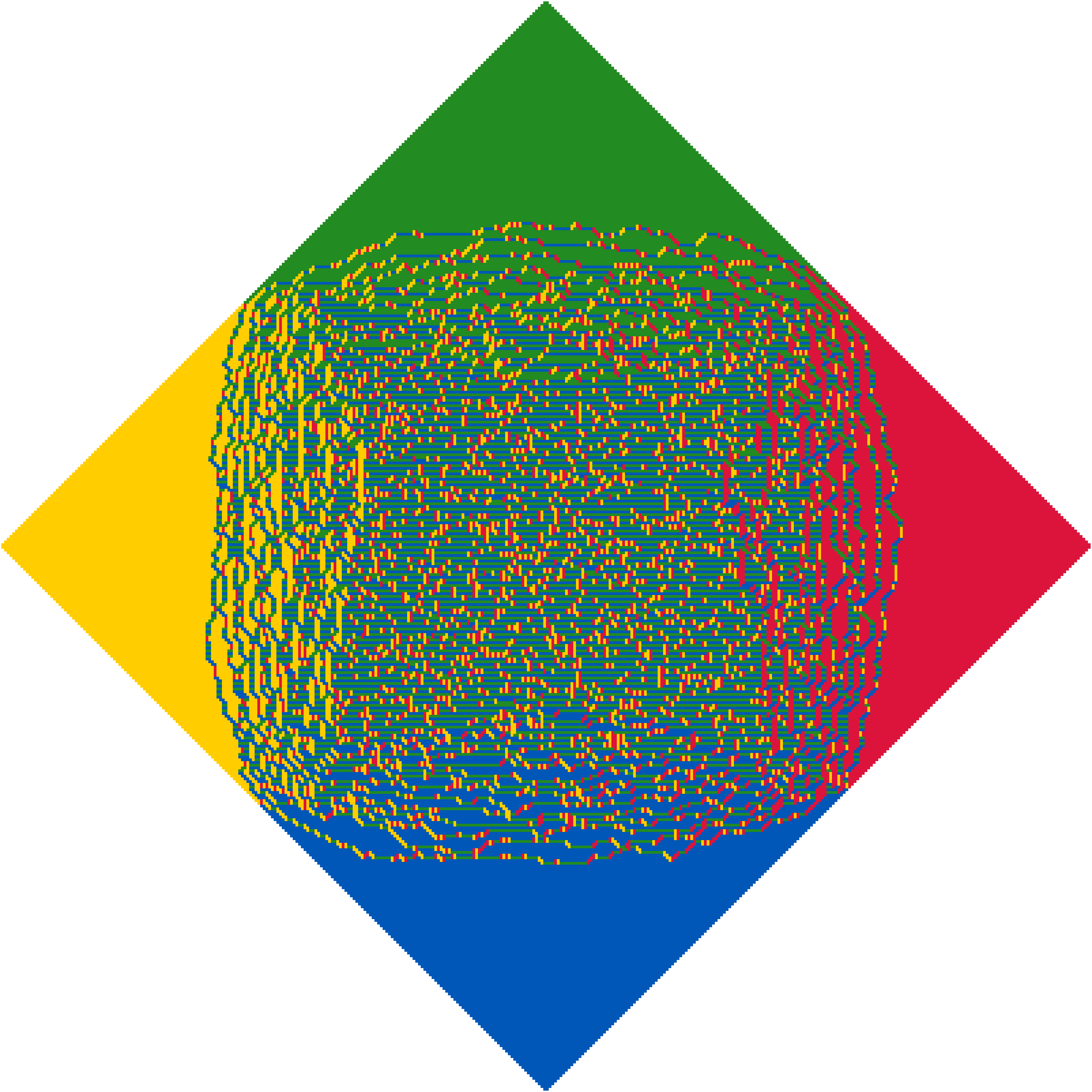
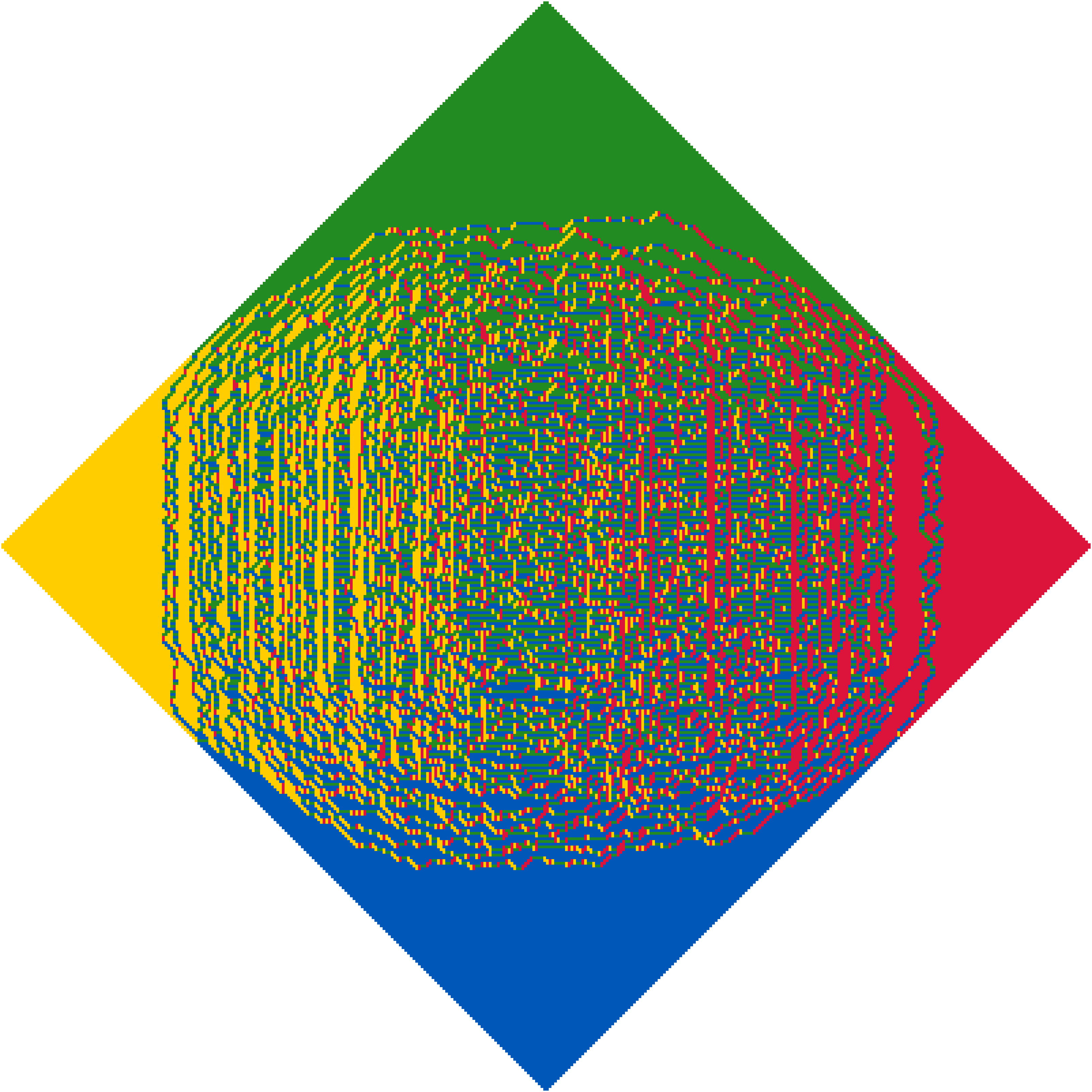
Diagonally Layered Disorder

Model:
Sample i.i.d. parameters \(\boldsymbol\beta_1,\ldots,\boldsymbol\beta_M\in(0,1)\). The nontrivial edge weight in diagonal layer \(j\) is
\(\displaystyle W_j=\frac{\boldsymbol\beta_j}{1-\boldsymbol\beta_j}\)
Unlabeled edges have weight \(1\). The raw weights \(W_j\) may be heavy-tailed.
Probability measure:
\(\displaystyle \mathbf{P}(D) = \frac{1}{Z} \prod_{e \in D} \operatorname{weight}(e)\)
Two regimes as \(M \to \infty\): [Bufetov–P.–Zografos 2025]
  1. Critical vanishing variance:
    \(M\operatorname{Var}(\boldsymbol\beta_j)\to\sigma^2\), \(\boldsymbol\beta_j\to\beta\).
    Same limit shape as deterministic \(W=\beta/(1-\beta)\). Global/moment covariance: GFF + Brownian term.
  2. Fixed law of \(\boldsymbol\beta_j\), independent of \(M\).
    New limit shape from \(\mathcal B\). Global moments scale \(\sqrt{M}\), with Brownian-in-level covariance.
One-periodic weights on the Aztec diamond

Schur Generating Functions for Random Environment

Schur generating function [Gorin–Panova 2012], [Bufetov–Gorin 2013]:
\(\displaystyle S_{\rho}(u_1,\ldots,u_N) = \sum_{\lambda} \rho(\lambda) \frac{s_\lambda(u_1,\ldots,u_N)}{s_\lambda(1^N)}\)
where \(\rho\) is the distribution of a partition \(\lambda\), and \(u_j \in \mathbb{C}\)
For random environment [Bufetov–P.–Zografos 2025]:
The annealed SGF has an explicit product form (\(M\) is the size of the Aztec diamond, \(N\) is the level):
\(\displaystyle \begin{aligned} S_{\rho_N}(x_1,\ldots,x_N) &= \operatorname{\mathbf E}_{\boldsymbol{\mathcal B}_M} \prod_{j=N+1}^{M}\prod_{i=1}^{N} (1-\boldsymbol\beta_j+x_i\boldsymbol\beta_j) \\ &=\left(\operatorname{\mathbf E}_{\boldsymbol{\mathcal B}_M} \prod_{i=1}^{N}(1-\boldsymbol\beta+x_i\boldsymbol\beta) \right)^{M-N}. \end{aligned} \)
where \(\boldsymbol\beta,\boldsymbol\beta_j\sim\boldsymbol{\mathcal B}_M\) are independent, and the raw edge weight is \(W=\boldsymbol\beta/(1-\boldsymbol\beta)\). No moment assumptions on \(W\): it can be heavy-tailed.
Asymptotics of the \(N\)-th root of the SGF as \(N\to\infty\) yield LLN and CLT for the height function of the domino tilings.
Domino tiling to particle correspondence

Limit Shapes Under Random Weights

Limit shape equation:
\((\alpha, y) \in [0,1]^2\) are coordinates in the Aztec diamond. Solve for \(z\) in the upper half-plane:
\(\displaystyle \frac{z}{z-1} + (\alpha^{-1}-1) z \, \mathbf{E}_{\mathcal B}\frac{W}{1+W z} = \alpha^{-1} y\)
(recall \(W=\boldsymbol\beta/(1-\boldsymbol\beta)\))
Limiting density:
\(\displaystyle (\alpha,y)\mapsto \frac{1}{\pi}\,\mathrm{Arg}\bigl(z(\alpha,y)\bigr)\)
Arctic curve is the locus of double roots in \(z\), and we take real \(z\) as the parametrization of the frozen boundary.
Arctic curve for Bernoulli random weights
Bernoulli
\(\tfrac12\) and \(5\)
Arctic curve for uniform random weights
Uniform
\(W_i \sim [0,2]\)
Sampling...

Diagonal Disorder

Annealed: Brownian motion [Bufetov–P.–Zografos 2025]
pre-sampled
Quenched: GFF [Berestycki–Laslier–Ray 2016], [Zografos 2025]
pre-sampled
Diagonal disorder, \(W_i \sim \mathrm{Uniform}[0,2]\), \(N=1000\)

Straight-Layered Disorder

Straight-layered disorder: i.i.d. weights along horizontal layers — a 45° rotation from the diagonal case. \(W_i=0.3\) or \(5\) with prob \(\tfrac{1}{2}\). [Moulard–Toninelli 2025, arXiv:2507.11964, on torus]: studied singularities of the free energy, showed correlations decay as \(e^{-\sqrt{\text{distance}}}\) instead of polynomially.
Strictly periodic
pre-sampled
Gauge equivalent to 2×2 periodic model [Chhita–Johansson 2014]
Random layered
pre-sampled

IID Gamma-Distributed Weights

Model: [Duits–Van Peski 2025, arXiv:2512.03033]
\(\alpha\) edges \(\sim \Gamma(\alpha, 1)\), \(\beta\) edges \(\sim \Gamma(\beta, 1)\). Gamma is the unique distribution preserved by the shuffling algorithm. Turning point fluctuations scale as \(n^{2/3}\) (vs \(n^{1/2}\) for deterministic weights). Connection to integrable polymers (log-Gamma, strict-weak).
pre-sampled
\(\alpha = 0.2, \beta = 0.25\)
pre-sampled
\(\alpha = 1.0, \beta = 1.0\)

Summary

QR code for lpetrov.cc/lozenge-draw/
lpetrov.cc/lozenge-draw/
Draw a shape and tile by lozenges