Random Surfaces from Stacking Cubes:
A Visual Journey
University of Virginia
Loading...
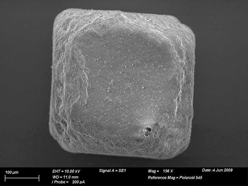
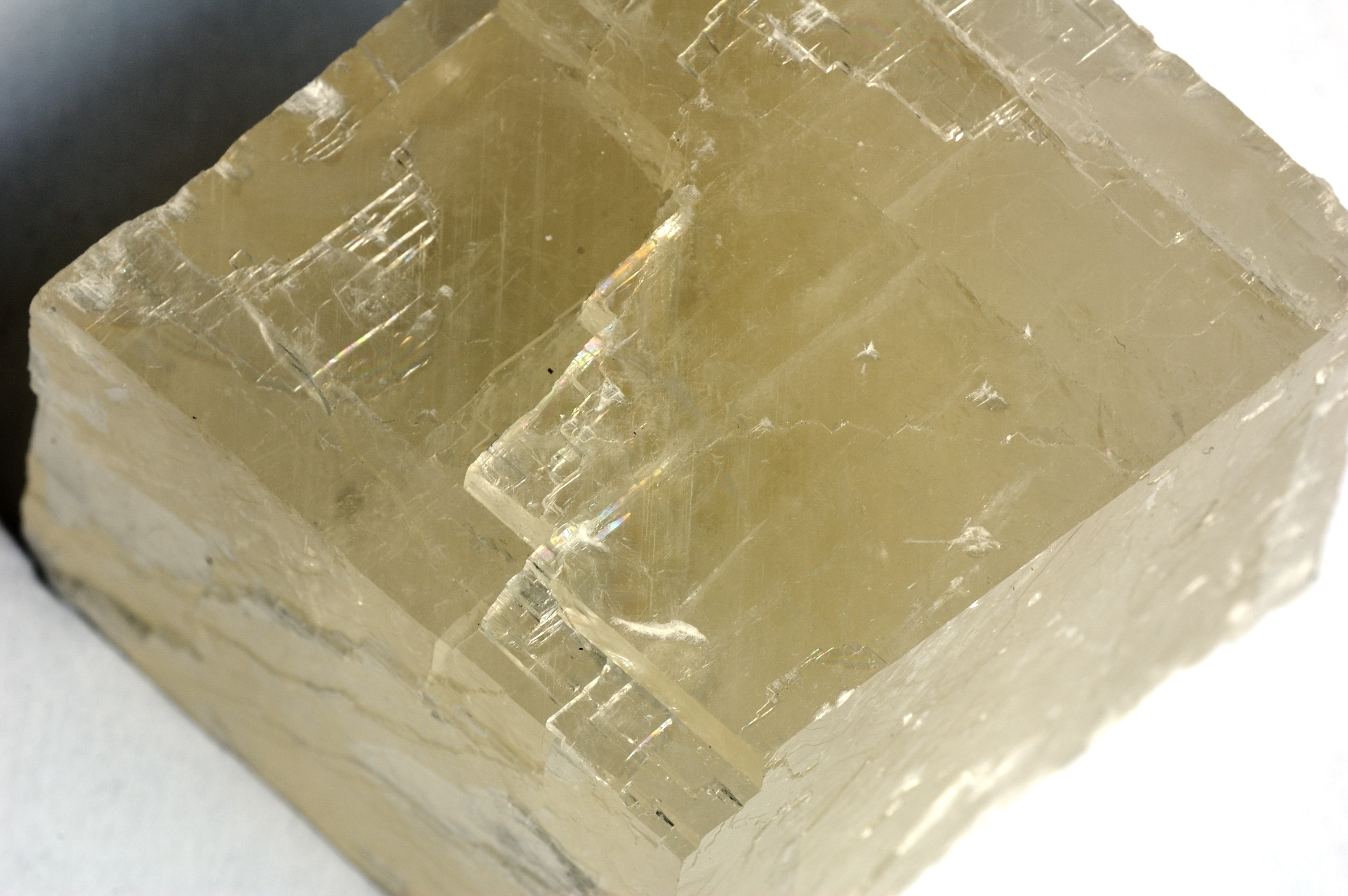
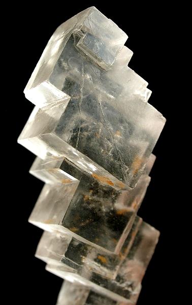
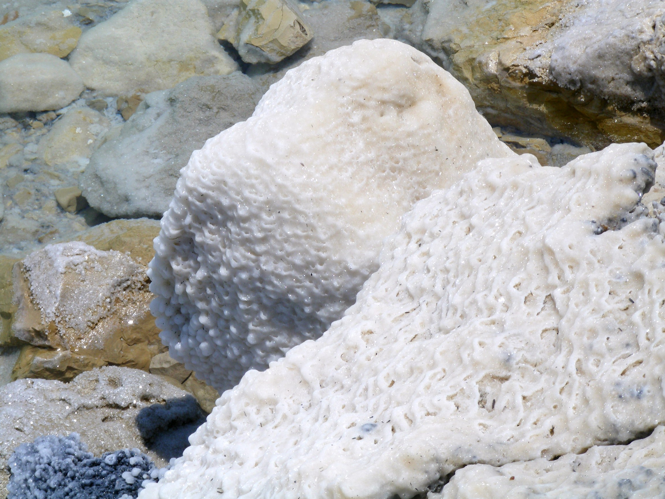
How Does Nature Make Shape?
Salt — same substance with cubic crystal structure, at different scales and growth conditions
Mathematical (random) crystal growth
How can something random have a predictable shape?
3.6
(q = 0.990)
a = 180, b = 135 · Loading...
Zoomed in: local segment
Locally, paths don't know about the global weight — still IID Bernoulli!
Why?
The limit shape maximizes entropy minus γ × area.
This yields IID Bernoulli with position-dependent \(p\) = slope of the limit shape.
The weight only affects the global shape, not the local behavior.
-->
What Else Can We Tile by Lozenges?
Non-simply-connected
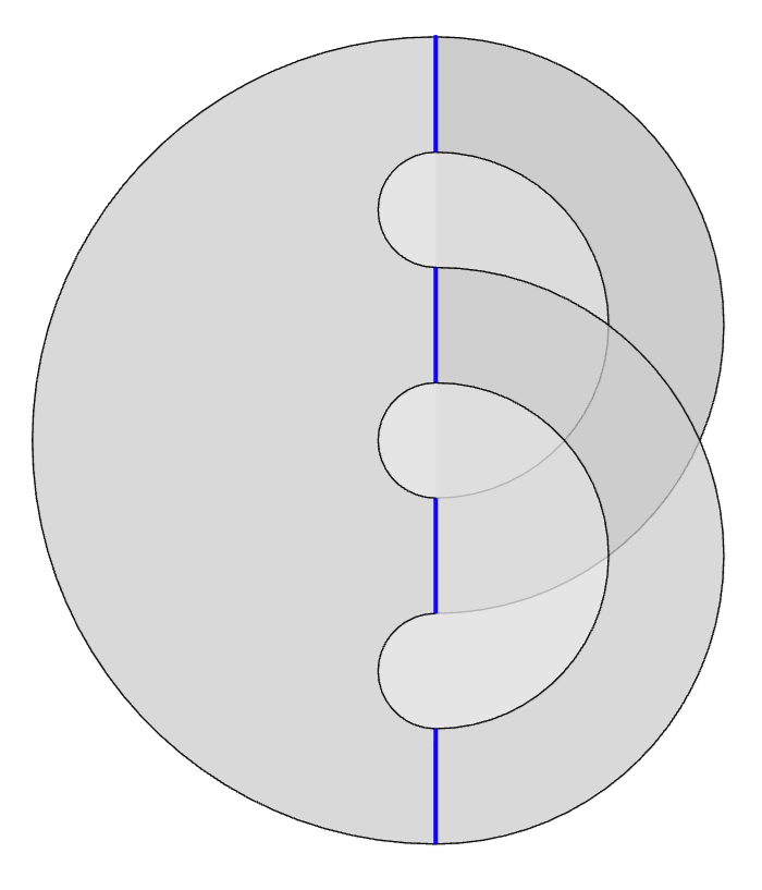
Non-planar orientable
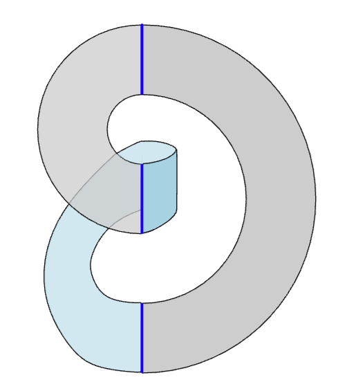
Non-orientable (Möbius strip)
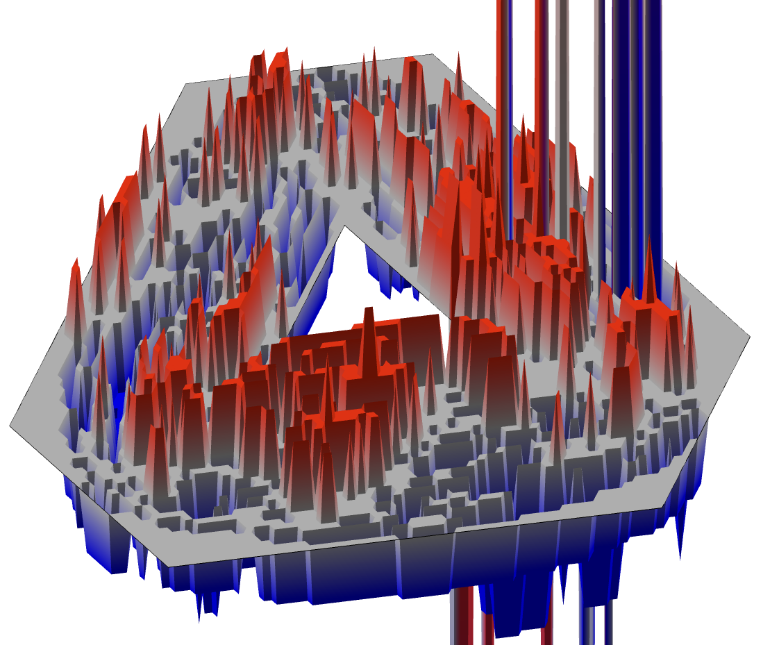
State of the art
[Borot–Gorin–Guionnet 2026]: Universal Gaussian fluctuations for some non-simply-connected, non-planar, or non-orientable domains.
Fluctuations for generic simply-connected domains: still open!
Fluctuations for generic simply-connected domains: still open!
Exact Sampling: We need to know when to stop waiting
Coupling From The Past (CFTP)
[Propp–Wilson 1996]
Surfaces are partially ordered by height function. The Markov chain is monotone, so it suffices to track just the maximal and minimal chains.
- The stationary chain is somewhere in between the maximal and minimal surfaces
- Run coupled dynamics — when max and min coalesce, we've caught the stationary chain
- To ensure exactness, use the backward-doubling protocol: start chains at times \(-1, -2, -4, -8, \ldots\) and check coupling at time \(0\)
- Output is an exact sample from the stationary distribution
Not approximately random — EXACTLY random.
Compare with calculus: we know \(1/n \to 0\), but for which \(n\) is it equal to zero?
Here we reach the limit exactly — but at a random time.
Here we reach the limit exactly — but at a random time.
Hexagon 35 × 35 × 35

draw any border and lozenge tile! (plus 3D printing exports)
lpetrov.cc/lozenge-draw (opens in new tab)