Continuous space TASEP     TASEPs

Simulation of a continuous-space TASEP on the positive real line. Particles enter at the boundary and jump distances following exponential distributions. The visualization studies Gaussian fluctuation behavior near bottleneck points.

The model [1]

The continuous space TASEP is a continuous time Markov process $\{X(t)\}_{t\ge 0}$ on the space

of finite particle configurations on $\mathbb R_{>0}.$ The particles are ordered, and the process preserves this ordering. However, more than one particle per site it allowed.

The Markov process $X(t)$ on $\mathcal{X}$ depends on the following data:

• Distance parameter $L>0$ (in asymptotic regimes we consider this parameter will grow to infinity);
• Speed function $\xi(y),$ $y\in \mathbb R_{\geq 0},$ which is assumed to be positive, piecewise continuous, have left and right limits, and uniformly bounded away from $0$ and $+\infty;$
• Discrete set $\mathbf{B}\subset \mathbb R_{>0}$ without accumulation points and such that there are only finitely many points of $\mathbf{B}$ in a right neighborhood of $0$. Fix a function $p: \mathbf B\rightarrow (0,1)$.

The process $X(t)$ evolves as follows:

• New particles enter $\mathbb R_{>0}$ (leaving $0$) at rate $\xi(0)$ (we say that a certain event has rate $\mu>0$ if it repeats after independent random time intervals which have exponential distribution with rate $\mu$ (and mean $\mu^{-1}$));
• If at some time $t>0$ there are particles at a location $x \in R_{>0}$, then one particle decides to leave this location at rate $\xi(x)$ (these events occur independently for each occupied location). Almost surely at each moment in time only one particle can start moving;
• The moving particle (say, $x_j$) instantaneously jumps to the right by some random distance $x_j(t)-x_j(t-)=\min(Y, x_{j-1}(t-)-x_j(t-))$ (by agreement, $x_0\equiv+\infty$). The distribution of $Y$ is as follows: $ Prob (Y \geq y ) = e^{-L y}\prod\limits_{b \in \mathcal{\mathbf B}, \text{ }x_j(t-)<b<x_j(t-)+y} p(b). $

This model is a $q=0$ degeneration of the one studied in [2].

Sampling algorithm

The simulation is straightforward. In continuous time, we choose which particle jumps, then increase the continuous time count by the corresponding exponential random variable, and perform the necessary comparisons.

Data file format

The data files are integer arrays like

{0.0286274477178, 0.0286274477178, 0.210833155189, }

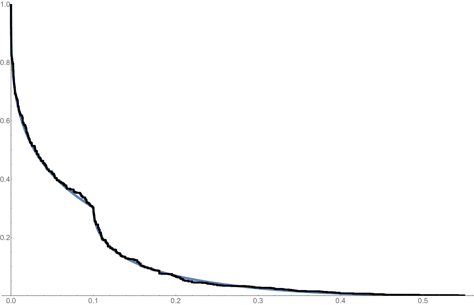
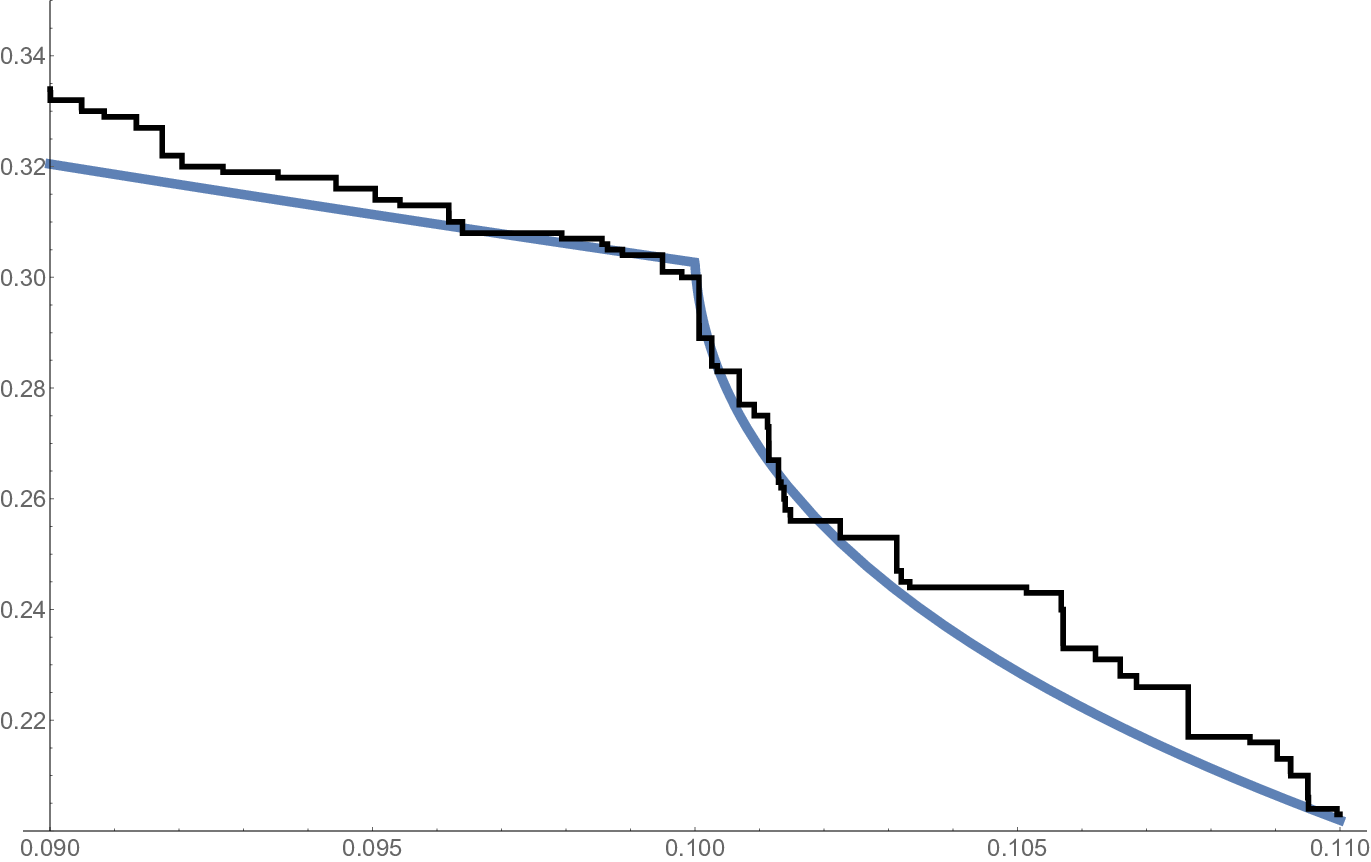
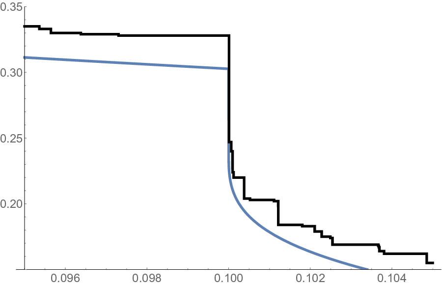
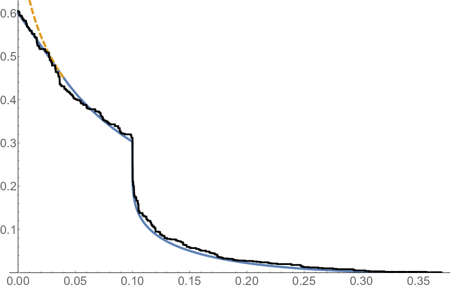
of particle locations. The plots display the height function (rescaled) which counts the number of particles to the right of a given location. In some plots the theoretical limit shape is also given.

code

• Link to code (python2 for simulations, simple Mathematica for drawing. Mathematica source not present)

1. Fully homogeneous case • (data: 15 KB) • (graphics: 14 KB)

   $t=1000, \xi(x)\equiv 1$
   

2. Fully homogeneous case with limit shape • (data: 15 KB) • (graphics: 16 KB)

   $t=1000, \xi(x)\equiv 1$
   

3. Mild slowdown (about critical) • (data: 16 KB) • (graphics: 17 KB)

   $t=1000, \xi(x)=\mathbf{1}_{x<0.1}+\frac12\mathbf{1}_{x\ge 0.1}$
   

4. Mild slowdown (about critical), zoom around the slowdown • (data: 16 KB) • (graphics: 13 KB)

   $t=1000, \xi(x)=\mathbf{1}_{x<0.1}+\frac12\mathbf{1}_{x\ge 0.1}$
   

5. Harder slowdown • (data: 15 KB) • (graphics: 16 KB)

   $t=1000, \xi(x)=\mathbf{1}_{x<0.1}+0.3\cdot\mathbf{1}_{x\ge 0.1}$
   

6. Harder slowdown, zoom around the slowdown • (data: 15 KB) • (graphics: 12 KB)

   $t=1000, \xi(x)=\mathbf{1}_{x<0.1}+0.3\cdot\mathbf{1}_{x\ge 0.1}$
   

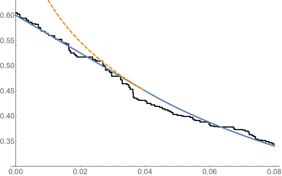
7. Slower initial stream of particles (roadblock in the beginning) • (data: 9 KB) • (graphics: 15 KB)

   Gaussian behavior for $0 < x < 0.04$. Dashed curve is the limit shape with full initial stream of particles.
   $t=1000, \xi(x)= 0.6\cdot\mathbf{1}_{x=0}+\mathbf{1}_{0 < x<0.1}+0.3\cdot\mathbf{1}_{x\ge 0.1} $
   

8. Slower initial stream of particles (roadblock in the beginning), zoom around the Gaussian behavior • (data: 9 KB) • (graphics: 13 KB)

   Gaussian behavior for $0 < x < 0.04$. Dashed curve is the limit shape with full initial stream of particles.
   $t=1000, \xi(x)= 0.6\cdot\mathbf{1}_{x=0}+\mathbf{1}_{0 < x<0.1}+0.3\cdot\mathbf{1}_{x\ge 0.1} $
   

references

1. A. Knizel, L. Petrov, A. Saenz. In preparation (2018)
2. A. Borodin, L. Petrov, Inhomogeneous exponential jump model (2017), Probability Theory and Related Fields, to appear • https://arxiv.org/abs/1703.03857 (opens in new tab)

Dear colleagues: