Simulation showing the backwards evolution of TASEP. The particle system is first simulated forward to time T, then evolved backwards. The movie visualization demonstrates that the distribution at each time matches the original forward distribution.
This is a simulation illustrating the main result from the paper in preparation [1].
Multitime distributions
In addition to the dynamical simulation (the movie below), we can generate joint pictures of the height function at different times. Here are the ones for TASEP:
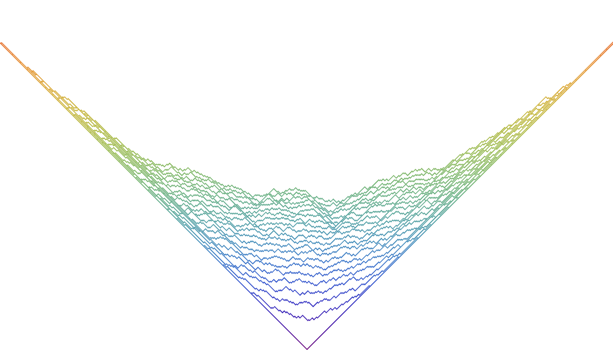
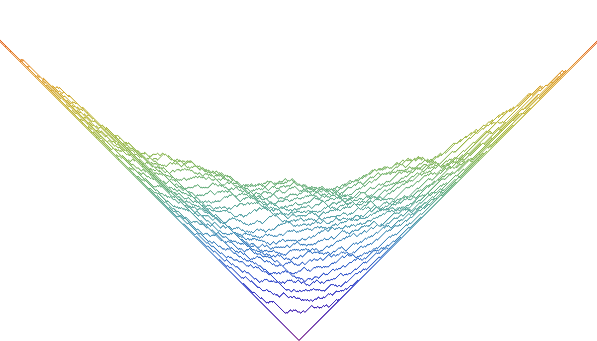
And for the backwards dynamics:
Data file format for the movie
The file contains Mathematica-readable array of the form ${t_i,H(t_i)}$, where $t_i$ are the timestamps, and $H(t_i)$ is the array of the values of the TASEP height function.
code
(note: parameters in the code might differ from the ones in simulation results below)-
Link to code(Code is available upon request)
-
Movie • (data: 125 MB) • (graphics: 1.8 MB)
Movie. TASEP goes forward up to time $t=350$. Then the configuration evolves according to the backwards dynamics, all the way down to (almost) time zero. The timestamps are shown on top. At each time during the backwards dynamics, the distribution of the random height function coincides with the one of the TASEP at the specified time moment.

references
- L. Petrov, A. Saenz. Mapping TASEP back in time (2019) • Probability Theory and Related Fields, 182, pages 481-530 (2022) • arXiv:1907.09155 [math.PR]