Simulations of stochastic higher spin vertex model
2015/03/12
The stochastic higher spin vertex model introduced in my paper with Ivan Corwin ([arXiv:1502.07374 [math.PR]][ivan6v]) generalizes the stochastic six vertex model considered by Borodin, Corwin, and Gorin, arXiv:1407.6729 [math.PR]. Here are some simulations related to this model.
Dear colleagues:
Feel free to use these pictures to illustrate your research in talks and papers, with attribution (CC BY-SA 4.0 (opens in new tab)). Some of the images are available in very high resolution upon request.
The stochastic higher spin vertex model generalizes a number of integrable stochastic particle systems on the line in the KPZ universality class:
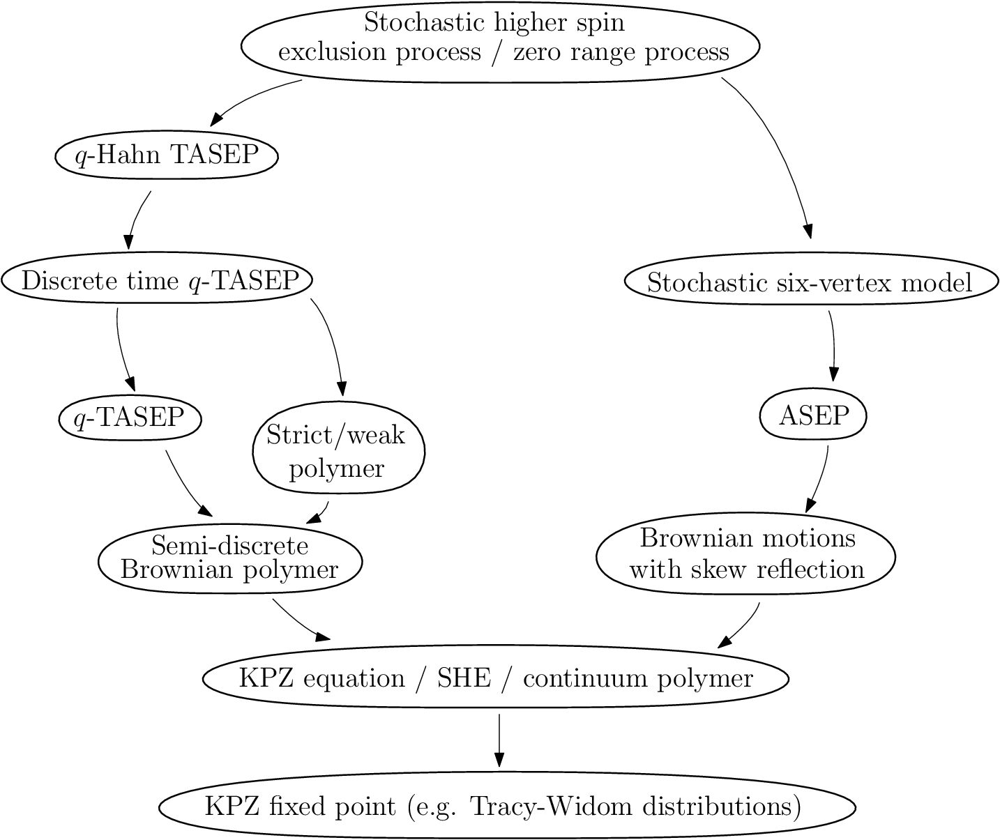 |
The stochastic higher spin vertex model is probabilistic, which puts probability weights on configurations of arrows in some region. In our interpretation, the arrows will always point up and to the right. We will take this region to be the integer quadrant \(\mathbb{Z}_{\ge0}^2\).
The model has 4 parameters: \(q\), \(\nu\), \(\alpha\), and \(J\). The simplest case of the model arises when \(J=1\). If \(J\) is a positive integer, then there are at most \(J\) horizontal arrows allowed.
Model in \(J=1\) case
Let us first explain how \(J=1\) probability weights are assigned at a single vertex. The numbers of incoming arrows at a vertex (bottom and left) \(i_1\) and \(j_1\) are interpreted as an input which is fixed, and then the probability weight is put on numbers of outgoing arrows \(i_2\) and \(j_2\), such that \(i_1+j_1=i_2+j_2\):
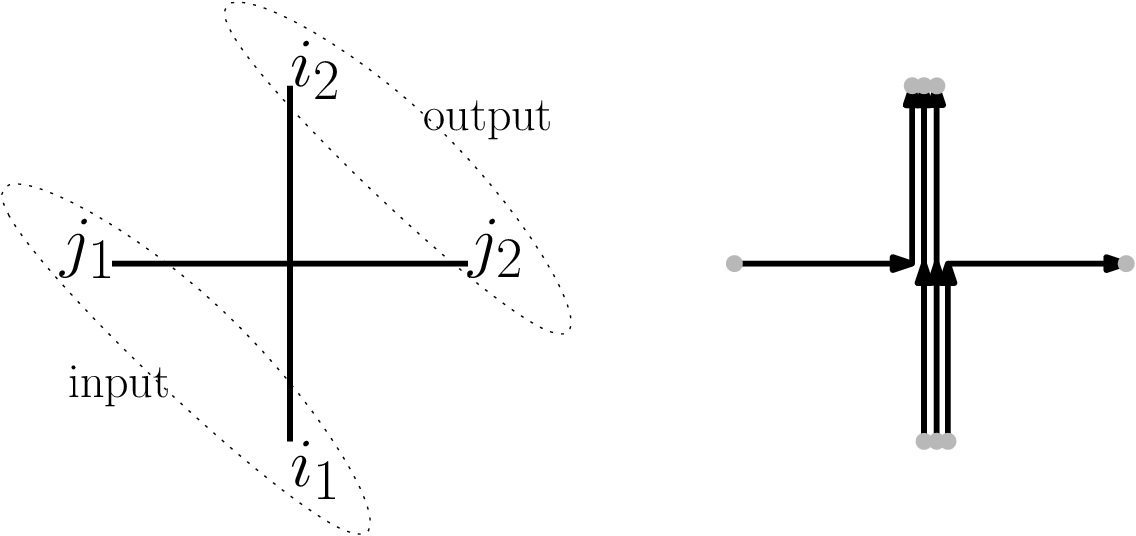 |
For \(J=1\), the probability weights have the following form (where \(g=0,1,2,\ldots\)):
 |
If \(\nu=q^{-I}\) for \(I=1,2,\ldots\), then an additional restriction arises: there are at most \(I\) vertical arrows allowed.
Starting from any boundary conditions on \(\mathbb{Z}_{\ge0}^2\), we can recursively sample the configuration of arrows.
Simulations in \(J=1\) case
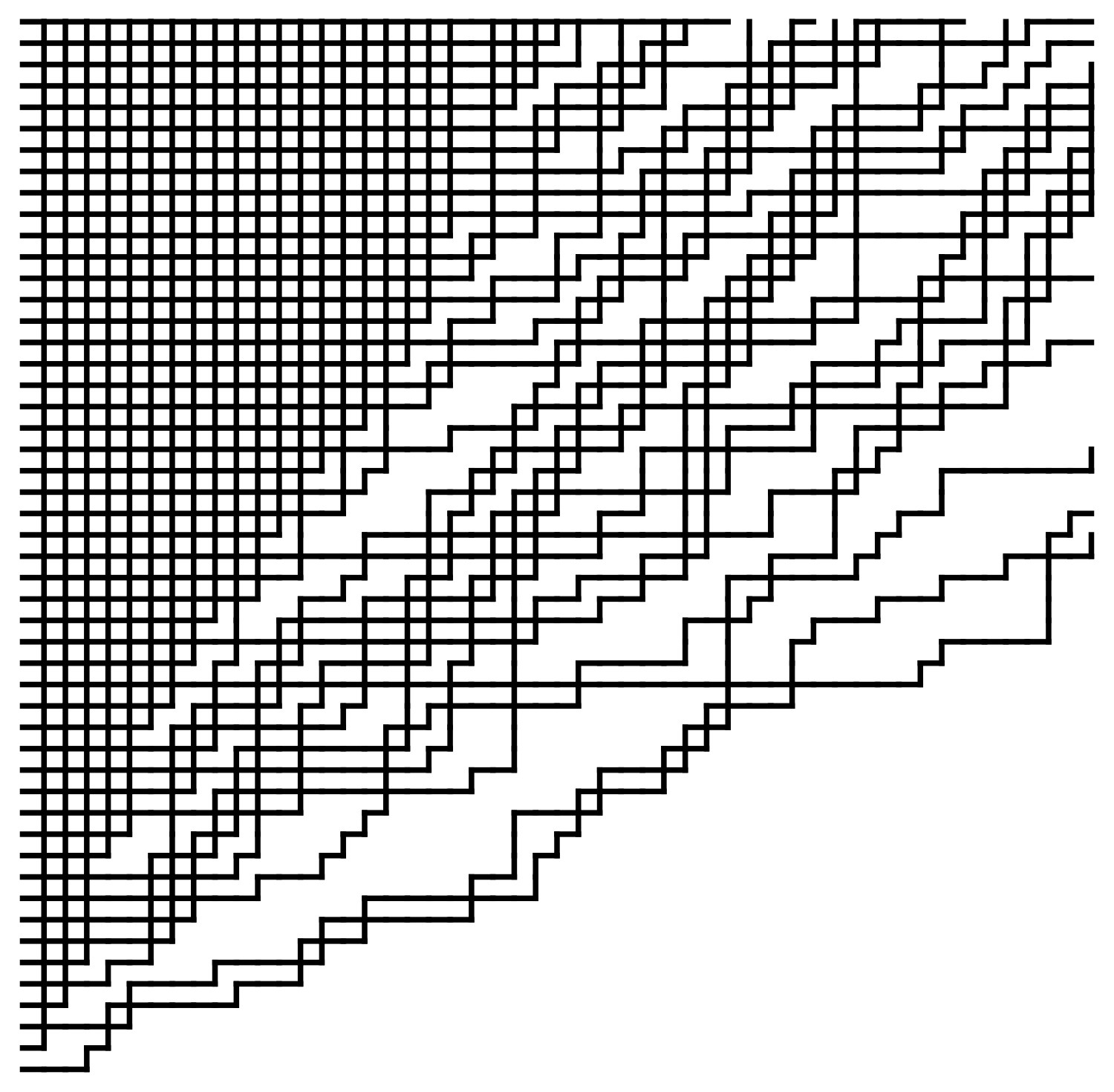
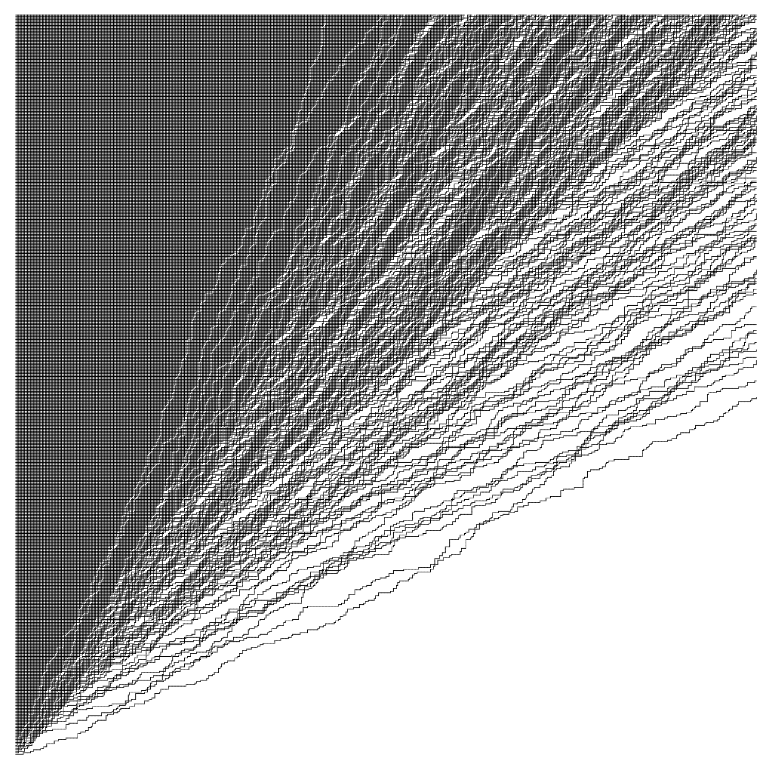
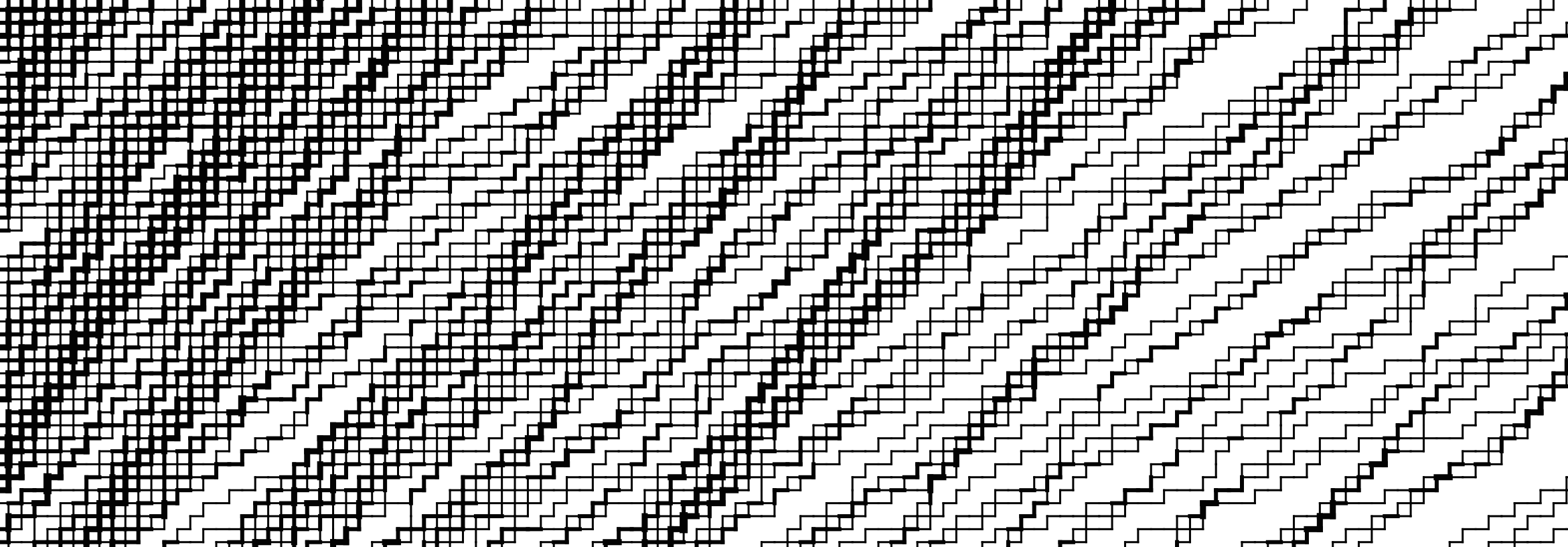
We choose the boundary conditions to consist of all incoming arrows from the left, and no incoming arrows from the bottom. In simulations below, the arrows are drawn without arrowheads, and thickness of an edge represents the number of arrows at that edge.
Stochastic six vertex model $(I=J=1)$
The limit shape and KPZ fluctuations theorems for the six vertex model were proven in arXiv:1407.6729 [math.PR].
 |
 |
 |
 |
$I=4$, $J=1$
 |
 |
General \(\nu\) and \(J=1\)
 |
 |
 |
Model in general \(J\) case
For an integer \(J\), the vertex weights may be obtained by a fusion procedure (first performed by Kirillov and Reshetikhin; J. Phys. A, 1987), by putting \(J=1\) layers with changing parameters: \(\alpha, q\alpha, q^2\alpha, \ldots, q^{J-1}\alpha\). For example, for \(J=2\) we obtain the following vertex weights:
 |
In general, the vertex weights can be expressed through the basic hypergeometric functions, and, moreover, are always polynomials in \(q^J\). Therefore, one can perform an analytic continuation in \(q^J\), and regard \(J\) (or rather \(q^J\)) as a complex parameter. However, for \(J\) not integer, resulting systems in general fail to become stochastic. There is at least one stochastic system which can be obtained via this analytic continuation, it arises at \(\alpha=-\nu\), \(q^J\alpha=-\mu\), and it is the \(q\)-Hahn system introduced by Povolotsky in arXiv:1308.3250 [math-ph].
Simulations in general \(J\) case
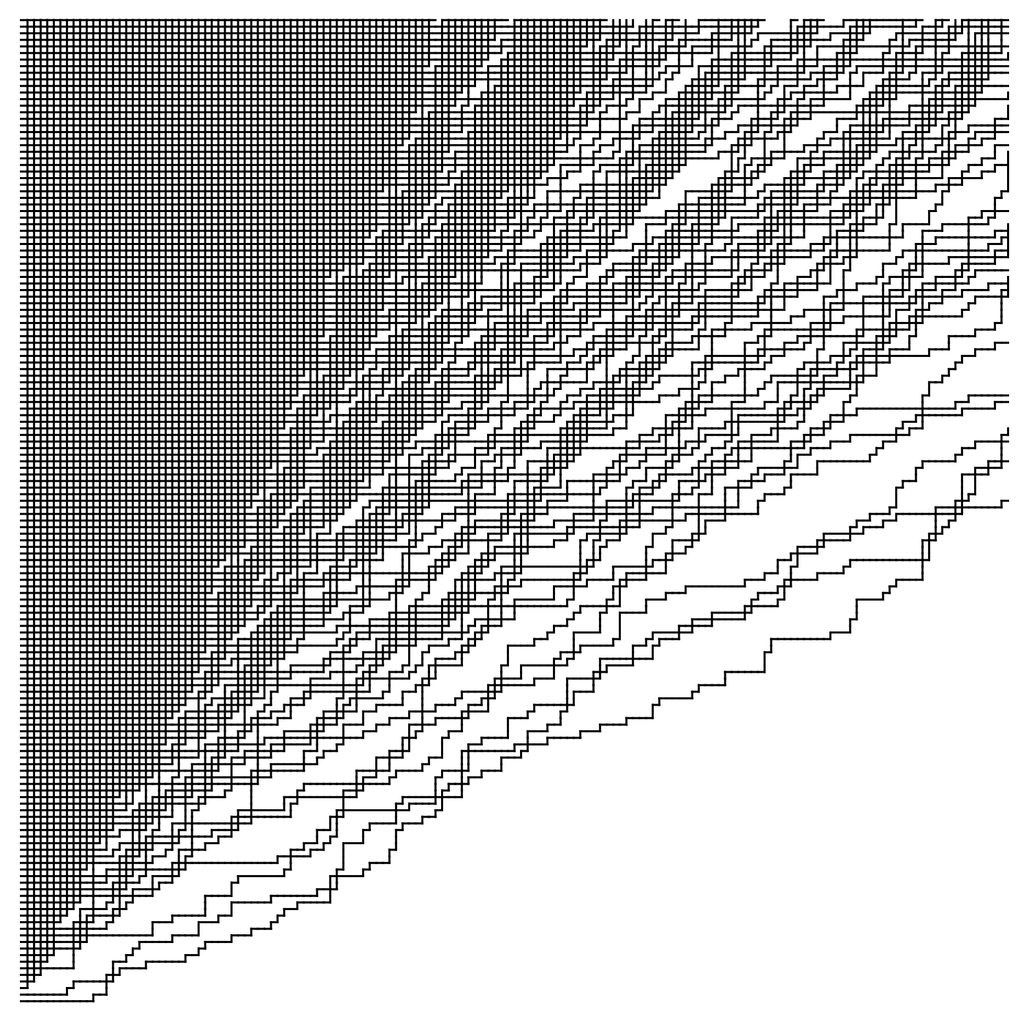
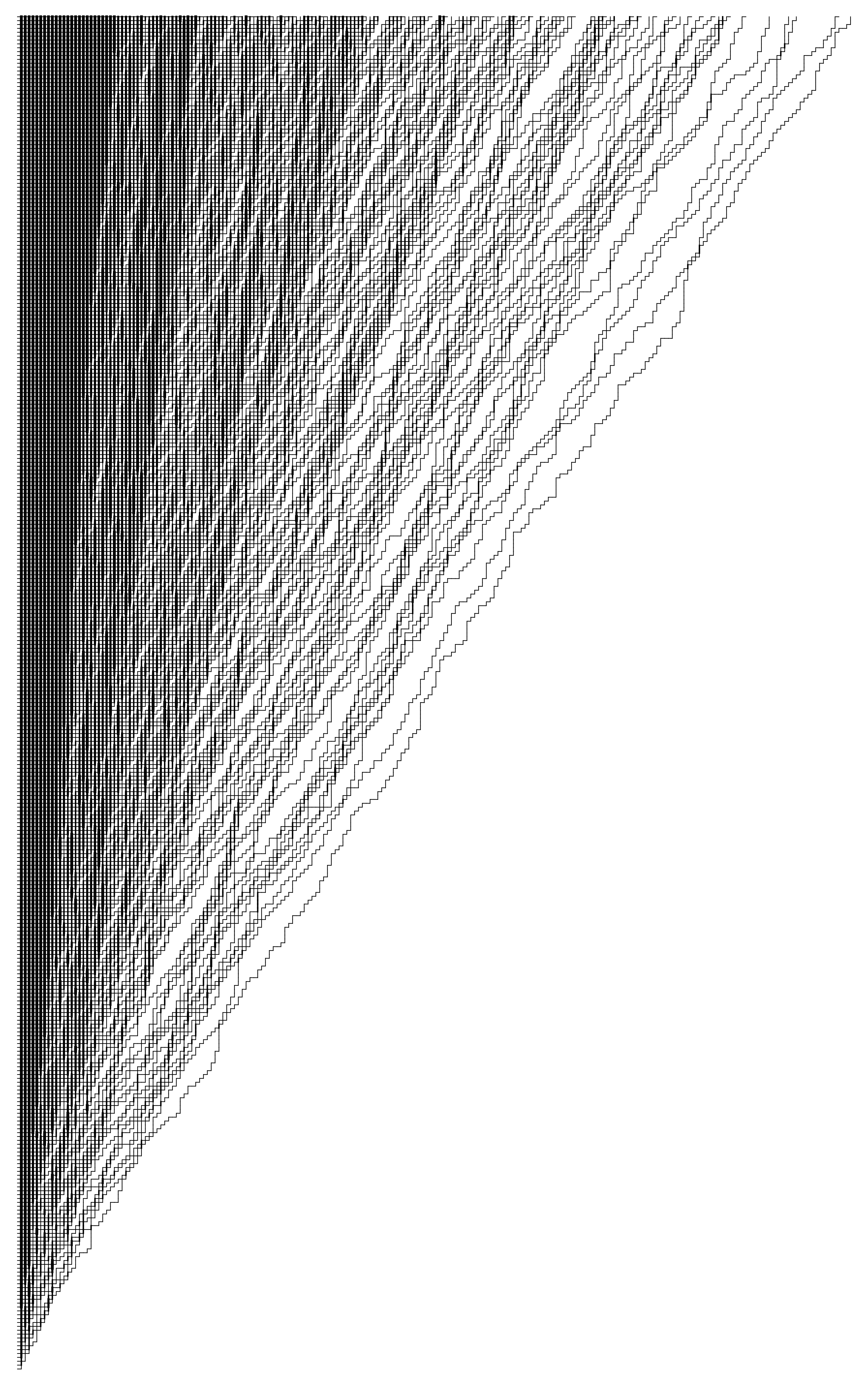
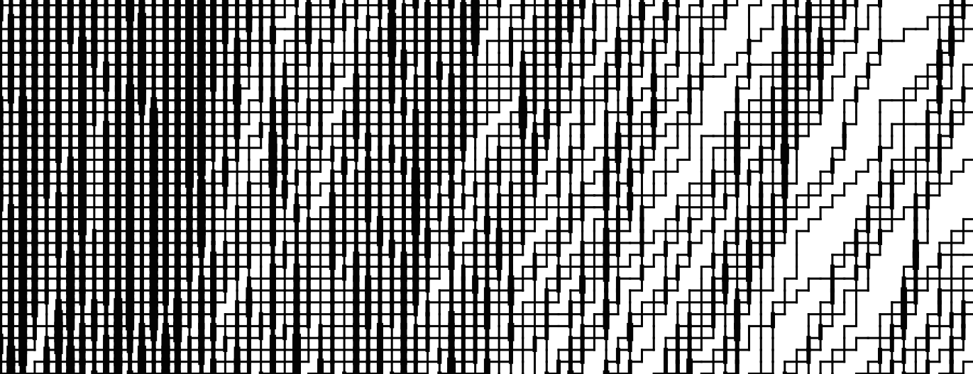
We choose the boundary conditions to consist of \(J\) incoming arrows from the left, and no incoming arrows from the bottom. In simulations below, the arrows are drawn without arrowheads, and thickness of an edge represents the number of arrows at that edge.
 |
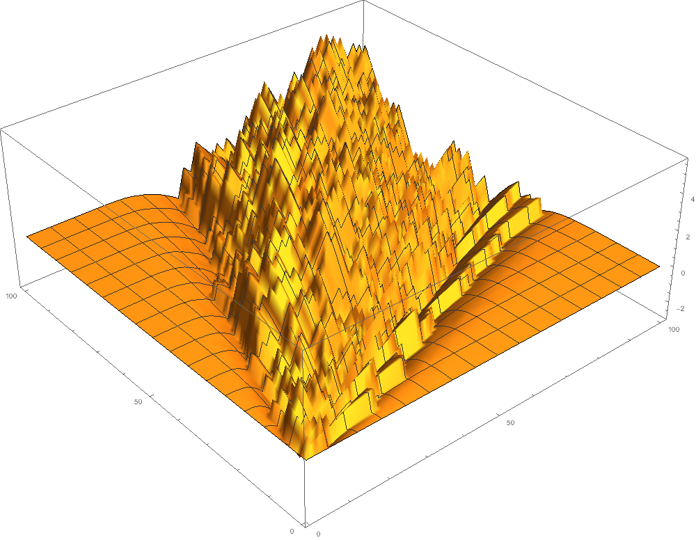
 |
Fluctuations of the stochastic six vertex model